In this tutorial we'll cover everything you need to know about web scraping using the R programming language. We'll explore the ecosystem of R packages for web scraping, build complete scrapers for real-world datasets, tackle common challenges like JavaScript rendering and pagination, and even analyze our findings with some data science magic. Let's get started!
Hearing web scraping for the first time? Take a quick detour to our Web Scraping Fundamentals guide. It covers all the basics, history, and common use cases that will help you build a solid foundation before diving into R-specific implementations. If you're a newbie, consider it your must-read primer!
The 8 Key Packages in R Web Scraping for 2025
When I first started scraping with R, I felt overwhelmed by the number of packages available. Should I use rvest? What about httr? Is RSelenium overkill for my needs? This section will save you from that confusion by breaking down the major players in the R web scraping ecosystem.
Let's start by comparing the most important R packages for web scraping:
| R Package | Status | Primary Use Case | Key Features | Best For |
|---|---|---|---|---|
| rvest | Active, maintained by the tidyverse team | Static HTML parsing | CSS/XPath selectors, form submission, table extraction | Beginner-friendly scraping of static websites |
| httr2 | Active, successor to httr | HTTP requests with advanced features | Authentication, streaming, async requests, response handling | API interactions, complex HTTP workflows |
| jsonlite | Active, widely used | JSON parsing and manipulation | Converting between JSON and R objects | Working with API responses, JSON data |
| xml2 | Active, maintained by the tidyverse team | XML/HTML parsing | XPath support, namespace handling | Low-level HTML/XML manipulation |
| RCurl | Less active, older package | Low-level HTTP handling | Comprehensive cURL implementation | Legacy systems, specific cURL functionality |
| Rcrawler | Maintained | Automated web crawling | Parallel crawling, content filtering, network visualization | Large-scale crawling projects |
| RSelenium | Maintained | JavaScript-heavy websites | Browser automation, interaction with dynamic elements | Complex sites requiring JavaScript rendering |
| chromote | Active, well-maintained | JavaScript-heavy websites & anti-bot sites | Real Chrome browser automation, headless browsing, JavaScript execution | Modern websites with anti-scraping measures |
Let's briefly look at each of these in more detail.
- rvest: The rvest package, maintained by Hadley Wickham as part of the tidyverse, is the go-to choice for most R web scraping tasks. Inspired by Python's Beautiful Soup, it provides an elegant syntax for extracting data from HTML pages.
- httr2: The httr2 package is a powerful tool for working with web APIs and handling complex HTTP scenarios. It's the successor to the popular httr package and offers improved performance and a more consistent interface.
- jsonlite: When working with modern web APIs, you'll often receive data in JSON format. The jsonlite package makes parsing and manipulating JSON data a breeze.
- xml2: The xml2 package provides a lower-level interface for working with HTML and XML documents. It's the engine that powers rvest but can be used directly for more specialized parsing needs.
- RCurl: Before httr and httr2, there was RCurl. This package provides bindings to the libcurl library and offers comprehensive HTTP functionality. While newer packages have largely superseded it, RCurl still has its place for specific cURL features.
- Rcrawler: If your project requires crawling multiple pages or entire websites, Rcrawler offers specialized functionality for managing large-scale crawling operations, including parallel processing and network analysis.
- RSelenium: Some websites rely heavily on JavaScript to render content, making them difficult to scrape with standard HTTP requests. RSelenium allows you to control a real browser from R, making it possible to scrape dynamic content.
- chromote: The chromote package provides R with the ability to control Chrome browsers programmatically. Unlike RSelenium, it's lighter weight and doesn't require Java or external servers. It's perfect for scraping modern websites that depend heavily on JavaScript or implement anti-scraping measures that block simpler HTTP requests.
RSelenium deserves its own separate spotlight! If you're curious about this powerful browser automation tool, check out our comprehensive RSelenium guide. It covers everything from installation to advanced browser control techniques. Perfect for when you need industrial-strength scraping power or are building complex web automation workflows!
What This Guide Covers
In this tutorial, we'll focus primarily on using rvest, httr2, RCrawler, and chromote for our web scraping needs, as they represent the most modern and maintainable approach for most R scraping projects. Here's what we'll cover:
- Setting Up Your R Scraping Environment: Installing packages and understanding the basic scraping workflow
- Basic Scraping with rvest: Extracting content from static HTML pages
- Advanced HTTP handling with httr2: Managing headers, cookies, and authentication
- Complex Browser Automation with chromote: Handling JavaScript-heavy sites and bypassing common scraping blocks
- Handling Common Challenges: Working with JavaScript, pagination, and avoiding blocks
- Data Analysis: Scraping LEGO Racers data from BrickEconomy and exploring price trends and value factors
Whether you're an R programmer looking to add web scraping to your toolkit or a data scientist tired of copying numbers by hand, this guide has you covered. Let's dive in and liberate your data!
Getting Started: Setting Up Your R Scraping Environment
Let's start by setting up your scraping lab! I remember my first scraping project - I spent more time wrestling with package installations than actually scraping data. Let's make sure you don't fall into the same pit.
Installing R and RStudio (If You Haven't Already)
If you're just getting started with R, you'll need both R (the actual programming language) and RStudio (an awesome interface that makes R much friendlier).
First, download and install R from CRAN:

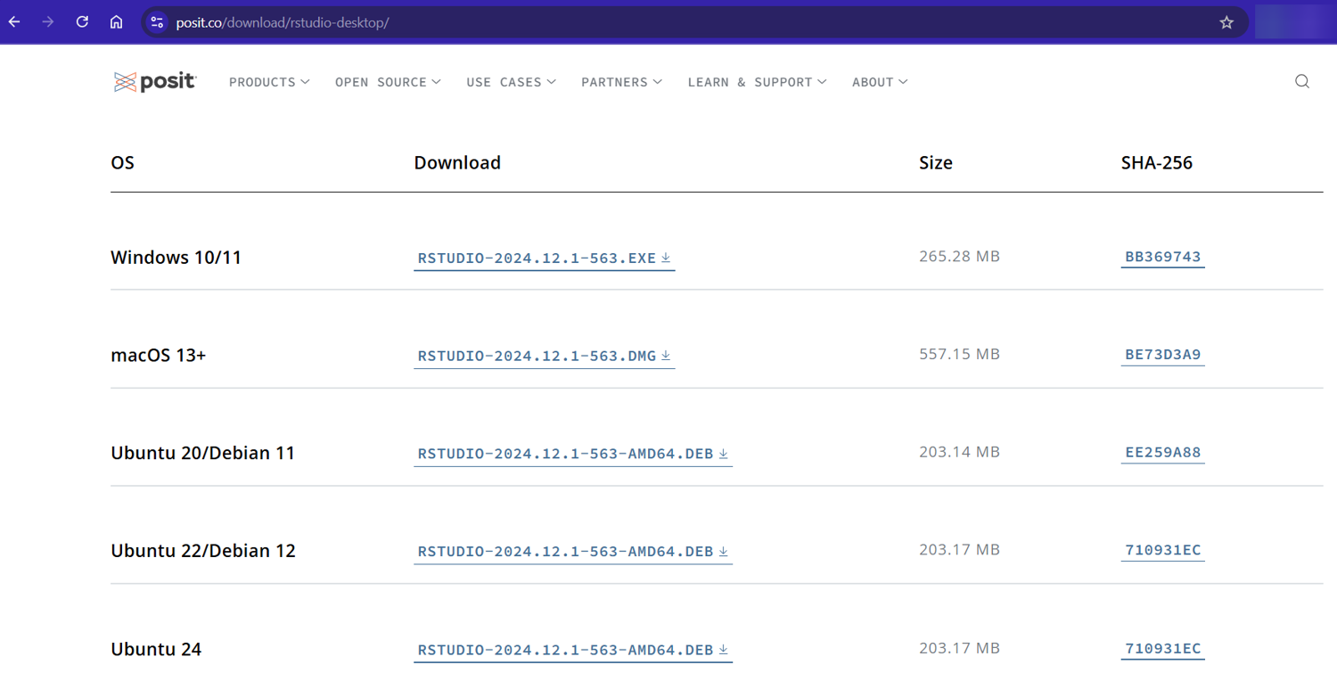
Next, download and install RStudio Desktop (the free version is perfect):
Installing R Scraping Packages
Once RStudio is up and running, you need to install the essential packages. You can do this directly from your terminal:
# On Linux/Mac terminal - install dependencies first
sudo apt update
sudo apt install libcurl4-openssl-dev libxml2-dev libfontconfig1-dev libfreetype6-dev
sudo apt install build-essential libssl-dev libharfbuzz-dev libfribidi-dev
sudo apt install libfreetype6-dev libpng-dev libtiff5-dev libjpeg-dev

# Then install the R packages
Rscript -e 'install.packages(c("tidyverse", "httr2", "jsonlite", "xml2", "rvest", "ragg"), repos="https://cloud.r-project.org", dependencies=TRUE)'
Running this installation script taught me the real meaning of patience. I've had time to brew coffee, reorganize my desk, and contemplate the meaning of life while waiting for R packages to compile. Consider it a built-in meditation break!
if you're on Windows or don't want to mess about with the terminal, please install Rtools you can find the installer here. Don't forget to add Rtools to your system path, the path might look like this:
C:\rtools40\usr\bin
Then open up Rstudio and run this in the console tab:
install.packages(c("tidyverse", "httr2", "jsonlite", "xml2", "rvest", "ragg"), repos="https://cloud.r-project.org", dependencies=TRUE)
When that's done, let's now create a new R script to make sure everything's working. From our terminal, we can use:
# Create a new R script
touch scraper.R
If you're a non-terminal user do this in RStudio instead:
File -> New File -> R Script
Now, let's load our scraping toolkit, paste this into the new file you created:
# Load the essential scraping packages
library(rvest)    # The star of our show - for HTML parsing
library(dplyr)    # For data wrangling
library(httr2)    # For advanced HTTP requests
library(stringr)  # For string manipulation

# Test that everything is working
cat("R scraping environment ready to go!\n")
Save this file and run it with Rscript scraper.R in your terminal. If you don't see any errors, you're all set!
R Web Scraping with rvest
Now that our environment is set up, let's dive into some practical examples using rvest. Think of rvest as your Swiss Army knife for web scraping – it handles most common scraping tasks with elegant, readable code.
Let's put our new tools to work! The theory is helpful, but nothing beats seeing real code in action. So let's start with some simple examples that demonstrate rvest's core functionality.
We'll start with the basics and gradually build up to more complex operations – the same progression I followed when learning web scraping myself.
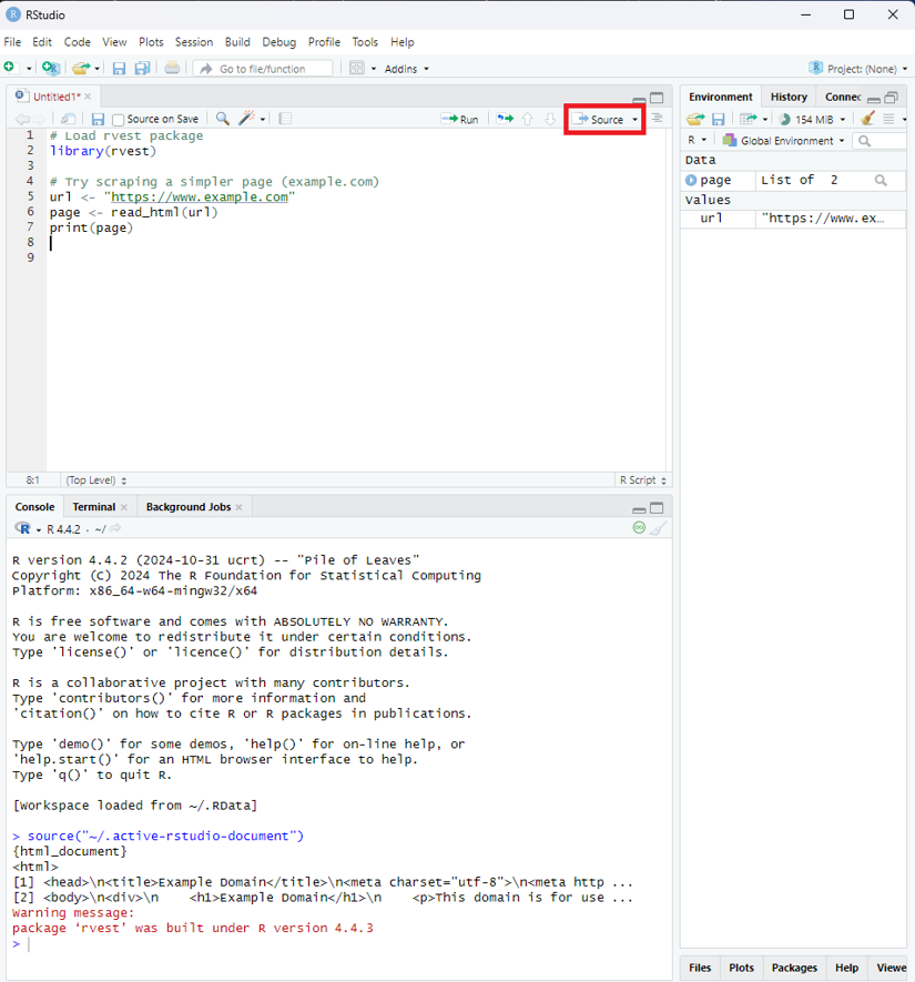
Example #1: Reading HTML
The first step in any web scraping workflow is fetching the HTML from a URL. The read_html() function makes this incredibly simple:
# Load rvest package
library(rvest)

# Read HTML from a URL
url <- "https://example.com"
page <- read_html(url)
print(page)

# You can also read from a local HTML file
# local_html <- read_html("path/to/local/file.html")
When I started scraping, I was amazed at how this single line of code could fetch an entire webpage. Under the hood, it's making an HTTP request and parsing the response into an XML document that we can work with.
If you're working in RStudio GUI, click the "source" to run your code.
Example #2: Selecting Elements With CSS Selectors
Once we have our HTML, we need to zero in on the elements containing our data. This is where CSS selectors shine:
# Extract all paragraph elements
paragraphs <- page %>% html_elements("p")

# Extract elements with a specific class
prices <- page %>% html_elements(".price")

# Extract an element with a specific ID
header <- page %>% html_elements("#main-header")
CSS and XPath selectors can be tricky to remember! Bookmark our XPath/CSS Cheat Sheet for quick reference. It's saved me countless trips to Stack Overflow when trying to target those particularly stubborn HTML elements!
I love how these selectors mirror exactly what you'd use in web development. If you're ever stuck figuring out a selector, you can test it directly in your browser's console with document.querySelectorAll() before bringing it into R.
Example #3: Extracting Text and Attributes
Now that we've selected our elements, we need to extract the actual data. Depending on what we're after, we might want the text content or specific attributes:
# Get text from elements
paragraph_text <- paragraphs %>% html_text2()

# Get attributes from elements (like href from links)
links <- page %>%
  html_elements("a") %>%
  html_attr("href")

# Get the src attribute from images
images <- page %>%
  html_elements("img") %>%
  html_attr("src")
The difference between html_text() and html_text2() tripped me up for weeks when I first started. The newer html_text2() handles whitespace much better, giving you cleaner text that often requires minimal processing afterward.
Example #4: Handling Tables
Tables are treasure troves of structured data, and rvest makes them a breeze to work with:
# Extract a table into a data frame
tables <- page %>% html_table()
first_table <- tables[[1]]  # Get the first table

# If you have multiple tables, you can access them by index
second_table <- tables[[2]]

# You can also be more specific with your selector
specific_table <- page %>%
  html_element("table.data-table") %>%
  html_table()
I once spent an entire weekend manually copying data from HTML tables before discovering this function. What would have taken days took seconds with html_table(). Talk about a game-changer!
Example #5: Navigating Between Pages
Real-world scraping often involves following links to collect data from multiple pages:
# Find links and navigate to them
next_page_url <- page %>%
  html_element(".pagination .next") %>%
  html_attr("href")

# If the URL is relative, make it absolute
if(!grepl("^http", next_page_url)) {
  next_page_url <- paste0("https://example.com", next_page_url)
}

# Now fetch the next page
next_page <- read_html(next_page_url)
}
This pattern is the backbone of web crawlers – following links from page to page to systematically collect data.
Pro Tip: I've learned the hard way that many websites use relative URLs (like "/product/123") instead of absolute URLs. Always check if you need to prepend the domain before navigating to the next page. This five-second check can save hours of debugging later. Check out our guide on How to find all URLs on a domain’s website for more insights.
Real-World rvest Example: Scraping IMDB Movie Data
Let's wrap up our rvest exploration with a real-world example. I love showing this to people new to web scraping because it perfectly demonstrates how a few lines of R code can unlock data that would take ages to collect manually.
For this example, we'll scrape IMDB to gather data about a particularly... unique cinematic achievement:
library(rvest)

# Let's scrape data about a cinematic masterpiece
movie_url <- "https://www.imdb.com/title/tt8031422/"
movie_page <- read_html(movie_url) # Read the main movie page

# First, let's grab the movie title
movie_title <- movie_page %>%
  html_element("h1") %>%
  html_text2()

cat("Movie:", movie_title, "\n")
If you run this, you'll discover we're exploring "The Last Sharknado: It's About Time" (2018). Yes, I have questionable taste in movies, but great taste in scraping examples:
Pro Tip: CSS selectors are the secret language of web scraping success. Before going further, make sure you understand how to precisely target HTML elements with our comprehensive CSS Selectors guide. This skill is absolutely essential for writing efficient and maintainable scrapers!
Now, let's see who was brave enough to star in this film. From inspecting the page, the top cast members are listed in individual <div> elements. We need to select those elements and then extract the actor's name and character name from within each one using specific selectors (like data-testid attributes, which can be more stable than CSS classes):
# --- Extract Top Cast (from Main Page using Divs) ---
# Target the individual cast item containers using the data-testid
cast_items <- movie_page %>%
  html_nodes("[data-testid='title-cast-item']")

# Extract actor names from the specific link within each item
actor_names <- cast_items %>%
  html_node("[data-testid='title-cast-item__actor']") %>%
  html_text(trim = TRUE) # trim whitespace directly

# Extract character names similarly
character_names <- cast_items %>%
  html_node("[data-testid='cast-item-characters-link'] span") %>%
  html_text(trim = TRUE) # trim whitespace directly

# Combine actors and characters into a data frame
cast_df <- data.frame(
  Actor = actor_names,
  Character = character_names,
  stringsAsFactors = FALSE
)

# Display the full top cast list found
cat("\nCast (Top Billed):\n")
print(cast_df)
Running this code now extracts the actor and character names into a data frame. You'll still find a surprisingly star-studded cast in the results:
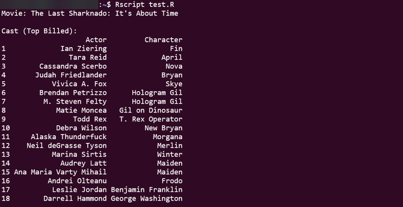
Ian Ziering (yes, the guy from Beverly Hills, 90210), Tara Reid (American Pie), and even cameos from Neil deGrasse Tyson and Marina Sirtis (Deanna Troi from Star Trek). Hollywood's finest clearly couldn't resist the allure of flying sharks!
But how good is this cinematic treasure? Let's scrape the rating:
rating <- movie_page %>%
  html_element("[data-testid='hero-rating-bar__aggregate-rating__score'] span:first-child") %>%
  html_text() %>%
  as.numeric()

cat("\nIMDB Rating:", rating, "/ 10\n")
# Output
IMDB Rating: 3.5 / 10
A stunning 3.5 out of 10! Clearly underrated (or perhaps accurately rated, depending on your tolerance for shark-based time travel chaos).
What I love about this example is how it demonstrates the core rvest workflow:
- Fetch the page with
read_html() - Select elements with
html_element()orhtml_nodes()(using CSS selectors or XPath) - Extract data with
html_text(),html_attr(), or sometimeshtml_table()(if the data is in an HTML table!) - Process as needed
Pro Tip: When building scrapers, I always start small by extracting just one piece of data (like the title) to make sure my selectors work. Once I've verified that, I expand to extract more data. This incremental approach saves hours of debugging compared to trying to build the whole scraper at once.
With these rvest basics in your toolkit, you can scrape most static websites with just a few lines of code. But what happens when websites use complex authentication, require custom headers, or need more advanced HTTP handling? That's where httr2 comes in!
Handling HTTP Requests in R with httr2
While rvest is perfect for straightforward scraping, sometimes you need more firepower. Enter httr2, the next-generation HTTP package for R that gives you fine-grained control over your web requests.
I discovered httr2 when I hit a wall trying to scrape a site that required specific headers, cookies, and authentication. What seemed impossible with basic tools suddenly became manageable with httr2's elegant request-building interface.
Example #1: Setting Headers and Cookies
Most serious websites can spot a basic scraper a mile away. The secret to flying under the radar? Making your requests look like they're coming from a real browser:
# Create a request with custom headers
req <- request("https://example.com") %>%
  req_headers(
    `User-Agent` = "Mozilla/5.0 (Windows NT 10.0; Win64; x64) AppleWebKit/537.36",
    `Accept-Language` = "en-US,en;q=0.9",
    `Referer` = "https://example.com"
  )

# Add cookies if needed
req <- req %>%
  req_cookies(session_id = "your_session_id")

# Perform the request
resp <- req %>% req_perform()

# Extract the HTML content
html <- resp %>% resp_body_html()
After spending days debugging a scraper that suddenly stopped working, I discovered the site was blocking requests without a proper Referer header. Adding that one header fixed everything! Now I always set a full suite of browser-like headers for any serious scraping project.
Example #2: Handling Authentication
Many valuable data sources hide behind login forms. Here's how to get past them:
# Basic authentication (for APIs)
req <- request("https://api.example.com") %>%
  req_auth_basic("username", "password")

# Or for form-based login
login_data <- list(
  username = "your_username",
  password = "your_password"
)

resp <- request("https://example.com/login") %>%
  req_body_form(!!!login_data) %>%
  req_perform()

# Save cookies for subsequent requests
cookies <- resp %>% resp_cookies()

# Use those cookies in your next request
next_req <- request("https://example.com/protected-page") %>%
  req_cookies(!!!cookies) %>%
  req_perform()
I once spent an entire weekend trying to scrape a site that used a complex authentication system. The breakthrough came when I used the browser's network inspector to see exactly what data the login form was sending. Replicating that exact payload in httr2 finally got me in!
Example #3: Rate Limiting and Retries
Being a good web citizen (and avoiding IP bans) means controlling your request rate and gracefully handling failures:
# Set up rate limiting and retries
req <- request("https://example.com") %>%
  req_retry(max_tries = 3, backoff = ~ 5) %>%
  req_throttle(rate = 1/3)  # Max 1 request per 3 seconds

# Perform the request
resp <- req %>% req_perform()
I learned about rate limiting the hard way. During my first large-scale scraping project, I hammered a site with requests as fast as my internet connection would allow. Five minutes later, my IP was banned for 24 hours. Now I religiously use req_throttle() to space out requests!
Example #4: Handling JSON APIs
Many modern sites use JSON APIs behind the scenes, even if they appear to be regular HTML websites:
# Make a request to a JSON API
req <- request("https://api.example.com/products") %>%
  req_headers(`Accept` = "application/json")

resp <- req %>% req_perform()

# Parse the JSON response
data <- resp %>% resp_body_json()

# Work with the data as a regular R list
product_names <- sapply(data$products, function(product) product$name)
Pro Tip: Some of the richest data sources I've found weren't visible HTML tables but hidden JSON APIs powering a website's frontend. Use your browser's network inspector to look for XHR requests when a page loads - you might find a cleaner data source than scraping HTML!
Example #5: Putting It All Together
Here's how a complete httr2 scraping workflow might look:
library(httr2)
library(rvest)

# Configure a base request template with all our common settings
base_req <- request("https://example.com") %>%
  req_headers(
    `User-Agent` = "Mozilla/5.0 (Windows NT 10.0; Win64; x64) AppleWebKit/537.36",
    `Accept-Language` = "en-US,en;q=0.9"
  ) %>%
  req_throttle(rate = 1/5) %>%  # Be polite!
  req_retry(max_tries = 3)      # Be persistent!

# Make a specific request
resp <- base_req %>%
  req_url_path_append("/products") %>%
  req_perform()

# Extract data using rvest on the response
html <- resp %>% resp_body_html()
product_names <- html %>%
  html_elements(".product-name") %>%
  html_text2()
The real power of httr2 comes from combining it with rvest. I use httr2 to handle all the HTTP complexities (headers, cookies, authentication) and then pass the response to rvest for the actual data extraction.
With these httr2 techniques in your arsenal, very few websites will remain off-limits to your scraping adventures.
Crawling Multiple Web Pages in R with Rcrawler
While rvest and httr2 excel at targeted scraping, sometimes you need to collect data from multiple pages or even entire websites. That's where Rcrawler shines - it's built for large-scale web crawling operations.
I discovered Rcrawler when working on a research project that required data from hundreds of interconnected pages. What would have taken days to code manually took just a few lines with Rcrawler.
library(Rcrawler)

# Basic website crawling
Rcrawler(Website = "https://example.com",
         no_cores = 4,  # Use 4 CPU cores for parallel crawling
         MaxDepth = 2)  # Only follow links 2 levels deep
But Rcrawler's real power comes from its targeted content extraction. Let's see it in action with a practical example.
Scraping Information from Wikipedia using R and Rcrawler
Imagine we're researching famous physicists and need their birth and death dates. Instead of visiting each Wikipedia page individually, we can automate the process with Rcrawler:
library(Rcrawler)
# List of scientists we're interested in
list_of_scientists <- c("Niels Bohr", "Max Born", "Albert Einstein", "Enrico Fermi")
# Create Wikipedia search URLs for each scientist
target_pages <- paste0('https://en.wikipedia.org/wiki/', gsub(" ", "_", list_of_scientists))
# Scrape specific data points using XPath patterns
scientist_data <- ContentScraper(
Url = target_pages,
XpathPatterns = c(
"//th[contains(text(), 'Born')]/following-sibling::td",
"//th[contains(text(), 'Died')]/following-sibling::td"
),
PatternsName = c("born", "died"),
asDataFrame = TRUE
)
# Display the results
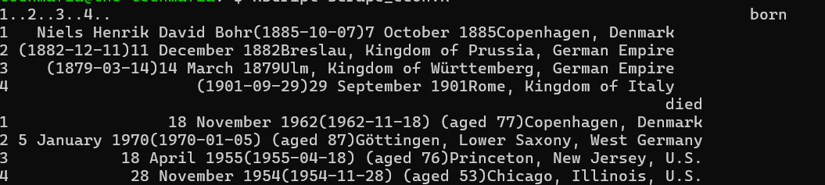
print(scientist_data)
When I first ran this code, I was amazed at how quickly it grabbed exactly the information I needed from multiple pages simultaneously. The result is a tidy data frame with birth and death information for each physicist - data that would have taken ages to collect manually:
Rcrawler can also visualize the link structure of websites using its NetworkData and NetwExtract parameters. I've used this to map customer journey paths through ecommerce data scraping and identify content silos in large websites. It's like getting an X-ray vision of a website's architecture:
# Crawl a site and extract its network structure
Rcrawler(Website = "https://small-website-example.com",
         no_cores = 2,
         NetworkData = TRUE,  # Extract network data
         NetwExtract = TRUE)  # Build the network graph

# This creates a file called "Net-Graph.graphml" that you can
# visualize with tools like Gephi or Cytoscape
While Rcrawler is incredibly powerful for broad crawling tasks, I generally prefer using rvest and httr2 for more targeted scraping jobs. Rcrawler's strengths come into play when you need to:
- Crawl many pages following a specific pattern
- Extract the same data elements from multiple similar pages
- Analyze the link structure of a website
- Parallelize crawling for better performance
Advanced Web Scraping in R: Using chromote for JavaScript-Heavy and Complex Sites
When websites detect and block simple HTTP requests (which is what rvest uses under the hood), it's time to bring out the big guns: browser automation. While many tutorials might want to point you to RSelenium at this point, I've found a much lighter and more elegant solution in the chromote package.
The beauty of chromote compared to RSelenium is that it's:
- Lightweight: No Java dependencies or Selenium server required
- Fast: Direct communication with Chrome DevTools Protocol
- Easy to install: Much simpler setup process
- Modern: Built for today's JavaScript-heavy websites
Let's see how chromote works!
Installing chromote and Chrome
First, we need to install both the R package and Chrome browser:
install.packages("chromote")
For the Chrome browser:
# Download the latest stable Chrome .deb package
wget https://dl.google.com/linux/direct/google-chrome-stable_current_amd64.deb

# Install the package (might require sudo)
sudo apt install ./google-chrome-stable_current_amd64.deb

# Clean up the downloaded file (optional)
# rm google-chrome-stable_current_amd64.deb

# If the install command complains about missing dependencies, try fixing them:
sudo apt --fix-broken install
Pro Tip: From my experience, if you're working on a headless server, you may need to install additional dependencies for Chrome. Running
sudo apt install -y xvfbhelps resolve most issues with running Chrome in headless environments.
Once you have both the chromote R package and the Google Chrome browser installed, your R environment is ready to start controlling the browser for advanced scraping tasks.
Practical Advanced Case Study: Scraping Datasets in BrickEconomy
You might be wondering, "Of all the websites in the world, why did you choose BrickEconomy for this tutorial?" Great question! When planning this guide, I had a choice to make: do I pick an easy target like a simple static website, or do I go for something that would actually challenge us and show real-world techniques?
BrickEconomy is perfect for teaching advanced scraping because it throws up nearly every obstacle a modern scraper will face in the wild. It has anti-bot protections, JavaScript-rendered content, pagination that doesn't change the URL, and nested data structures that require careful extraction. If you can scrape BrickEconomy, you can scrape almost anything!
Plus, let's be honest - scraping LEGO data is way more fun than extracting stock prices or weather data. Who doesn't want a dataset of tiny plastic race cars?
Now, let's build a scraper that:
- Finds all the LEGO Racers sets
- Extracts detailed information about each set
- Saves everything in a structured format
This collection provides a perfect case study. It has:
- Multiple pages of results (pagination challenges)
- Detailed information spread across multiple sections
- A mix of text, numbers, and percentages to parse
- Modern anti-scraping protections that require a real browser
This project will showcase advanced techniques that you can apply to almost any web scraping task in R.
Exploring BrickEconomy's Web Structure
Before we dive into code, let's take a moment to understand the structure of BrickEconomy's pages. This step is crucial for any scraping project—the better you understand the site structure, the more robust your scraper will be.
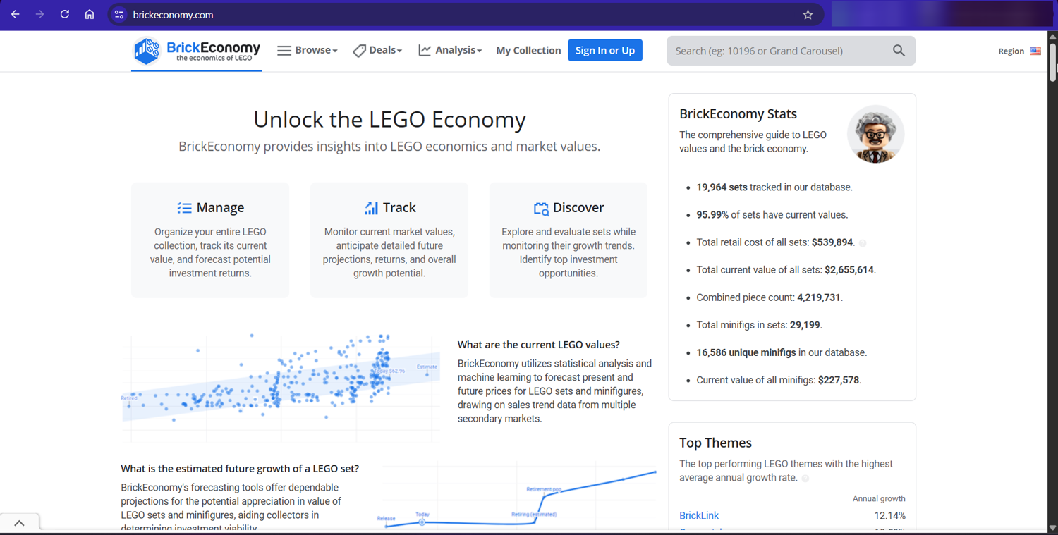
Theme page we're interested in: https://www.brickeconomy.com/sets/theme/racers

Let's break down what we're seeing:
- There's a paginated table of LEGO sets
- Each set has a link to its detail page
- Navigation buttons at the bottom allow us to move through pages
- The site uses JavaScript for navigation (the URL doesn't change when paging)
When we inspect an individual set page, like the Enzo Ferrari, we find:
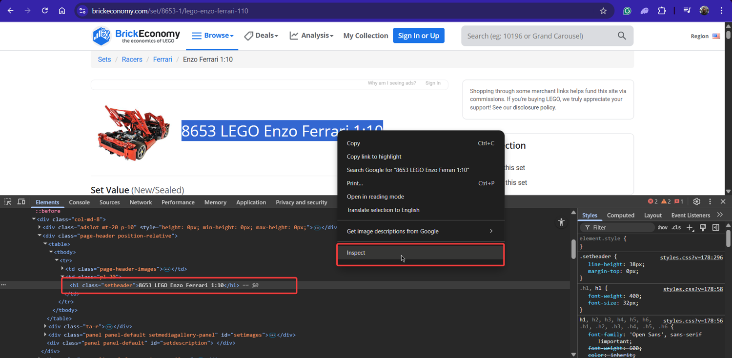
The data we want is organized in several sections. As we can see:
- The set title in an
<h1>tag - Set details (number, pieces, year) in a section with class
.side-box-body - Pricing information in another
.side-box-bodywith additional class.position-relative
After carefully inspecting the HTML, we can identify the selectors we need:
| Data | CSS Selector | Notes |
|---|---|---|
| Set Links | table#ContentPlaceHolder1_ctlSets_GridViewSets > tbody > tr > td:nth-child(2) > h4 > a | From the sets listing page |
| Next Button | ul.pagination > li:last-child > a.page-link | For pagination |
| Set Title | h1 | From individual set pages |
| Set Details Section | .side-box-body | Contains "Set number"; multiple exist |
| Detail Rows | div.rowlist | Within the details section |
| Row Keys | div.col-xs-5.text-muted | Left column in each row |
| Row Values | div.col-xs-7 | Right column in each row |
| Pricing Section | .side-box-body.position-relative | Contains pricing information |
Our scraper will have two main functions:
get_all_set_urls()- Collects all the LEGO Racers set URLs by navigating through paginationscrape_set_details()- Visits each URL and extracts detailed information
Let's break these down with code snippets and explanations.
Step #1: Setting Up Our Environment
Like any R project, we start by loading the necessary packages and defining key variables we'll use throughout the script:
# --- Step 1: Libraries and Configuration ---

print("Loading libraries...")
# Install packages if needed
# install.packages(c("chromote", "rvest", "dplyr", "stringr", "purrr", "jsonlite"))

# Load necessary libraries
suppressPackageStartupMessages({
  library(chromote) # For controlling Chrome
  library(rvest)    # For parsing HTML
  library(dplyr)    # For data manipulation (used in bind_rows)
  library(stringr)  # For string cleaning
  library(purrr)    # For list manipulation (used by helper function check)
  library(jsonlite) # For saving JSON output
})
print("Libraries loaded.")

# --- Configuration ---
start_url <- "https://www.brickeconomy.com/sets/theme/racers" # Target page
base_url <- "https://www.brickeconomy.com"                   # Base for joining relative URLs
ua_string <- "Mozilla/5.0 (Windows NT 10.0; Win64; x64) AppleWebKit/537.36 (KHTML, like Gecko) Chrome/108.0.0.0 Safari/537.36" # User agent
timeout_ms <- 60000 # 60 seconds for navigation/load events
wait_timeout_seconds <- 30 # Max wait for page update after pagination click
polite_sleep_range <- c(2, 5) # Min/max sleep seconds between scraping detail pages
max_pages_scrape <- 10 # Safety break for pagination loop (adjust if theme has more pages)
max_sets_scrape <- 2 # <<< SET LOW FOR TESTING, set to Inf for full run >>>
rds_url_file <- "racers_set_urls.rds"     # File to save/load intermediate URLs
rds_data_file <- "racers_set_data.rds"    # Final data output (RDS)
json_data_file <- "racers_set_data.json" # Final data output (JSON)

# --- End Step 1 ---
First up, we load our toolkit:
chromoteis the star for browser controlrvesthandles the HTML parsing once we have the content- dplyr and purrr provide handy data manipulation tools
- stringr helps clean up extracted text
- jsonlite allows us to save our results in the popular JSON format alongside R's native RDS format.
We also define filenames for saving our intermediate list of URLs (rds_url_file) and our final scraped data (rds_data_file, json_data_file). Notice the max_sets_scrape variable – keeping this low (like 2) is essential during testing to avoid scraping all 254 sets every time you run the code! Set it to Inf only when you're ready for the full run.
Step #2: Starting the URL Collection Function and Launching Chrome
Now we define the start of our first main function, get_all_set_urls, which handles finding all the individual set links from the paginated theme page. The first action inside is to launch the headless browser:
# --- Function Definition Start ---
get_all_set_urls <- function() {
  print("--- Function: get_all_set_urls ---")
  # Initialize variables for this function's scope
  all_relative_urls <- list()
  page_num <- 1
  navigation_success <- FALSE
  b <- NULL # Will hold our chromote session object

  # --- Step 2: Launch Browser ---
  tryCatch({
    b <- ChromoteSession$new() # Create the session (launches Chrome)
    print("Chromote session started for URL collection.")
  }, error = function(e) {
      print(paste("Error creating Chromote session:", e$message))
      # If session fails to start, return NULL (or empty list) from function
      return(NULL)
  })

  # Proceed only if session started successfully
  if (!is.null(b)) {
      # (Code for Step 3 and onwards goes here)
      # ...
  # --- End Step 2 ---  (Function continues)
We bundle the URL collection logic into a function for neatness. Inside, we initialize an empty list (all_relative_urls) to store the links we find. The core of this step is b <- ChromoteSession$new().
This single command tells chromote to launch an instance of Google Chrome running headlessly in the background and establish a connection to it, storing the connection object in the variable b. We wrap this in tryCatch so that if Chrome fails to launch for some reason (e.g., not installed correctly), the script prints an error and stops gracefully instead of crashing.
Step #3: Setting Up the Session and Initial Navigation
With the browser launched, we perform some initial setup within the session (like setting the User-Agent) and navigate to our starting page. We also set up an on.exit handler – a safety net to ensure the browser process is closed properly when the function finishes, even if errors occur later:
# (Continuing inside the 'if (!is.null(b))' block from Step 2)

    # --- Step 3: Initial Session Setup & Navigation ---
    # Ensure browser closes when function exits (even on error)
    on.exit({
        if (!is.null(b) && b$is_active()) {
            print("Closing URL collection session...")
            b$close()
        }
    })

    # Set the User-Agent for this session
    tryCatch({
      print("Setting User-Agent...");
      b$Network$setUserAgentOverride(userAgent = ua_string)
      print("User-Agent set.")
    }, error = function(e) {
        # Print warning but continue if UA fails
        print(paste("Error setting User-Agent:", e$message))
    })

    # Navigate to the first page of Racers sets
    print(paste("Navigating to:", start_url, "..."))
    tryCatch({
      b$Page$navigate(start_url, timeout = timeout_ms)
      print("Initial navigation successful.")
      navigation_success <- TRUE # Set flag for later steps
    }, error = function(e) {
        print(paste("Error during initial navigation:", e$message))
        navigation_success <- FALSE # Ensure flag is FALSE on error
    })
    # --- End Step 3 --- (Function continues)

    # if (navigation_success) { ... (Code for Step 4 goes here) }
Here, b$Network$setUserAgentOverride(...) tells the headless browser to send our specified ua_string with its requests, making it look more like a standard browser.
Next, b$Page$navigate(...) is the command that tells the browser to actually load the target URL. We again use tryCatch to handle potential navigation errors (e.g., website down, DNS issues) and set a navigation_success flag that we'll check before proceeding to scrape.
Step #4: URL Collection - Entering the Loop & Getting Page 1 HTML
Having successfully navigated to the first page, we now enter a loop to handle the pagination. The first thing inside the loop is to get the HTML content of the current page:
# (Continuing inside the 'if (!is.null(b))' block from Step 3)

    # Check if initial navigation was successful before starting loop
    if (navigation_success) {

      print("--- Starting Pagination Loop ---")
      # --- Step 4: Loop Start and Get Page HTML ---
      while(page_num <= max_pages_scrape) { # Loop until max pages or last page detected

        print(paste("Processing Page:", page_num))
        Sys.sleep(2) # Small pause for stability before interacting

        print("Getting HTML content...")
        html_content <- NULL # Reset variables for this iteration
        page_html <- NULL
        urls_from_current_page <- character(0)
        first_url_on_page <- NULL

        # Try to get the current page's HTML from chromote
        tryCatch({
          # Check session activity before commands
          if(is.null(b) || !b$is_active()) {
            print("Chromote session inactive during loop. Breaking.")
            break
          }
          # Get the root node of the document's DOM
          doc <- b$DOM$getDocument()
          root_node_id <- doc$root$nodeId
          # Get the full outer HTML based on the root node
          html_content_js <- b$DOM$getOuterHTML(nodeId = root_node_id)
          html_content <- html_content_js$outerHTML
          # Parse the retrieved HTML using rvest
          page_html <- read_html(html_content)
          print("HTML content retrieved and parsed.")

        }, error = function(e) {
            # If getting HTML fails, print error and stop the loop
            print(paste("Error processing page", page_num, ":", e$message))
            break # Exit while loop on error
        })

        # Check if HTML parsing failed silently (shouldn't happen if tryCatch works)
        if (is.null(page_html)) {
            print("Error: page_html is null after tryCatch. Stopping loop.")
            break
        }
        # --- End Step 4 --- (Loop continues)

        # (Code for Step 5 goes here)
        # ...
We first check our navigation_success flag from Step 3. Assuming we landed on page 1 okay, we start a while loop that will continue until we either hit the max_pages_scrape limit or detect the last page.
Inside the loop, after printing the current page number and a brief pause, we perform the crucial step of getting the page's source code. This isn't like httr; we need the HTML after the browser has potentially run JavaScript.
We use b$DOM$getDocument() and b$DOM$getOuterHTML() via chromote to grab the fully rendered HTML from the controlled Chrome instance. This raw HTML string (html_content) is then passed to rvest::read_html() to parse it into an xml_document object (page_html) that rvest can easily work with.
This whole sensitive operation is wrapped in tryCatch to handle potential errors during the interaction with the browser's DOM.
Step #5: URL Collection - Extracting URLs and Checking for End of Pages
With the parsed HTML for the current page (page_html), we can now extract the data we need: the set URLs. We also check if the "Next" button is disabled, indicating we've reached the last page:
# (Continuing inside the 'while' loop from Step 4)

        # --- Step 5: Extract URLs and Check for Last Page ---

        # Use the specific CSS selector to find set link elements
        set_link_selector <- "table#ContentPlaceHolder1_ctlSets_GridViewSets > tbody > tr > td:nth-child(2) > h4 > a"
        set_link_nodes <- html_elements(page_html, set_link_selector)

        # Extract the 'href' attribute (the relative URL) from each link node
        urls_from_current_page <- html_attr(set_link_nodes, "href")
        num_found <- length(urls_from_current_page)

        # Store the found URLs if any exist
        if (num_found > 0) {
            # Store the first URL to detect page changes later
            first_url_on_page <- urls_from_current_page[[1]]
            print(paste("Found", num_found, "URLs on page", page_num, "(First:", first_url_on_page, ")"))
            # Add this page's URLs to our main list
            all_relative_urls[[page_num]] <- as.character(urls_from_current_page)
        } else {
            # If no URLs found on a page (unexpected), stop the loop
            print(paste("Warning: Found 0 URLs on page", page_num, ". Stopping pagination."))
            break
        }

        # Check if the 'Next' button's parent li has the 'disabled' class
        print("Checking for 'Next' button state...")
        next_button_parent_disabled_selector <- "ul.pagination > li.disabled:last-child"
        disabled_check_nodes <- html_elements(page_html, next_button_parent_disabled_selector)

        # If the disabled element exists (length > 0), we are on the last page
        if (length(disabled_check_nodes) > 0) {
            print("Next button parent is disabled. Reached last page.")
            break # Exit the while loop
        }
        # --- End Step 5 --- (Loop continues if 'Next' is not disabled)

        # (Code for Step 6 goes here)
        # else { ... }
Here, we use rvest::html_elements() with the precise CSS selector we found during inspection (table#... a) to grab all the link nodes (<a> tags) for the sets listed on the current page.
Then, rvest::html_attr(..., "href") pulls out the actual URL from each link. We store the first URL found (first_url_on_page) so we can later check if the content has changed after clicking "Next". The list of URLs for this page is added to our main all_relative_urls list.
Crucially, we then check if the "Next" button is disabled. We look for its parent <li> element having the disabled class using the selector (ul.pagination > li.disabled:last-child) we found earlier. If html_elements finds such an element (length > 0), we know we're done, and we use break to exit the while loop.
Step #6: URL Collection - Clicking "Next" and Waiting Intelligently
If the "Next" button was not disabled, the script proceeds to the else block associated with the check in Step 5. Here, we simulate the click and then perform the vital "intelligent wait" to ensure the next page's content loads before the loop repeats:
# (Continuing inside the 'while' loop from Step 5)

        # --- Step 6: Click Next and Wait for Update ---
        else {
          # If 'Next' button is not disabled, proceed to click it
          print("'Next' button appears active.")

          # Define the selector for the clickable 'Next' link
          next_button_selector <- "ul.pagination > li:last-child > a.page-link"
          print(paste("Attempting JavaScript click for selector:", next_button_selector))

          # Prepare the JavaScript code to execute the click
          # We escape any quotes in the selector just in case
          js_click_code <- paste0("document.querySelector(\"", gsub("\"", "\\\\\"", next_button_selector), "\").click();")

          click_success <- FALSE # Flag to track if click worked
          # Try executing the JavaScript click
          tryCatch({
              b$Runtime$evaluate(js_click_code)
              print("JavaScript click executed.")
              click_success <- TRUE
            }, error = function(e) {
                print(paste("Error with JS click:", e$message))
                click_success <- FALSE
            })

          # If the click command failed, stop the loop
          if (!click_success) {
              print("JS click failed. Stopping.")
              break
          }

          # === Intelligent Wait ===
          print("Waiting for page content update...")
          wait_start_time <- Sys.time() # Record start time
          content_updated <- FALSE      # Flag to track if content changed

          # Loop until content changes or timeout occurs
          while (difftime(Sys.time(), wait_start_time, units = "secs") < wait_timeout_seconds) {
              Sys.sleep(1) # Check every second
              print("Checking update...")
              current_first_url <- NULL # Reset check variable

              # Try to get the first URL from the *current* state of the page
              tryCatch({
                  if(!b$is_active()) { stop("Session inactive during wait.") } # Check session
                  doc <- b$DOM$getDocument(); root_node_id <- doc$root$nodeId
                  html_content_js <- b$DOM$getOuterHTML(nodeId = root_node_id)
                  current_page_html <- read_html(html_content_js$outerHTML)
                  current_set_nodes <- html_elements(current_page_html, set_link_selector)
                  if (length(current_set_nodes) > 0) {
                      current_first_url <- html_attr(current_set_nodes[[1]], "href")
                  }
              }, error = function(e) {
                  # Ignore errors during check, just means content might not be ready
                  print("Error during wait check (ignored).")
              })

              # Compare the newly fetched first URL with the one from *before* the click
              if (!is.null(current_first_url) && !is.null(first_url_on_page) && current_first_url != first_url_on_page) {
                  print("Content updated!")
                  content_updated <- TRUE # Set flag
                  break # Exit the wait loop
              }
          } # End of inner wait loop

          # If the content didn't update within the timeout, stop the main loop
          if (!content_updated) {
              print("Wait timeout reached. Stopping pagination.")
              break
          }

          # Increment page number ONLY if click succeeded and content updated
          page_num <- page_num + 1

        } # End else block (if 'Next' button was active)
      } # End while loop (pagination)
      print("--- Finished Pagination Loop ---")

    } # End if (navigation_success)
# --- End Step 6 --- (Function continues to aggregate URLs)

# (Code for aggregating/saving URLs from get_all_set_urls goes here)
# ...
# } # End function get_all_set_urls
If the "Next" button is active, we prepare the JavaScript code needed to click it (document.querySelector(...).click();). We use b$Runtime$evaluate() to execute this JS directly in the headless browser. After triggering the click, the crucial "intelligent wait" begins. It enters a while loop that runs for a maximum of wait_timeout_seconds.
Here, we've successfully collected all the set URLs. Now, we need the logic to visit each of those URLs and extract the details. This involves two main parts:
- Defining the helper function that knows how to pull data from the detail page structure
- The main function that loops through our URLs and uses
chromoteto visit each page and call the helper function.
Step #7: Defining the Data Extraction Helper Function
Before looping through the detail pages, let's define the function responsible for extracting the actual data once we have the HTML of a set page. We'll design this function (extract_set_data) to actively identify the 'Set Details' and 'Set Pricing' sections before extracting the key-value pairs within them:
# --- Step 7: Define Data Extraction Helper Function ---

# This function takes parsed HTML ('page_html') from a single set page
# and extracts data from the 'Set Details' and 'Set Pricing' sections.
extract_set_data <- function(page_html) {
  set_data <- list() # Initialize empty list for this set's data

  # Try to extract the set title/heading (often in H1)
  title_node <- html_element(page_html, "h1")
  if (!is.null(title_node) && !purrr::is_empty(title_node)) {
    set_data$title <- str_trim(html_text(title_node))
    # print(paste("Extracted title:", set_data$title)) # Optional debug print
  } else {
    print("Warning: Could not extract title (h1 element)")
  }
Let's now start to extract the set details:
  # --- Extract Set Details ---
  # Strategy: Find all potential blocks, then identify the correct one.
  print("Attempting to identify and extract Set Details...")
  details_nodes <- html_elements(page_html, ".side-box-body") # Find all side-box bodies

  if (length(details_nodes) > 0) {
    found_details_section <- FALSE
    # Loop through potential sections to find the one containing "Set number"
    for (i in 1:length(details_nodes)) {
      row_nodes <- html_elements(details_nodes[[i]], "div.rowlist")
      contains_set_number <- FALSE
      # Check rows within this section for the key identifier
      for (row_node in row_nodes) {
        key_node <- html_element(row_node, "div.col-xs-5.text-muted")
        if (!is.null(key_node) && !purrr::is_empty(key_node)) {
          if (grepl("Set number", html_text(key_node), ignore.case = TRUE)) {
            contains_set_number <- TRUE
            break # Found the identifier in this section
          }
        }
      }

      # If this section contained "Set number", extract all data from it
      if (contains_set_number) {
        print("Found Set Details section. Extracting items...")
        found_details_section <- TRUE
        for (row_node in row_nodes) {
          key_node <- html_element(row_node, "div.col-xs-5.text-muted")
          if (!is.null(key_node) && !purrr::is_empty(key_node)) {
            key <- str_trim(html_text(key_node))
            if (key == "") next # Skip empty keys (like minifig image rows)

            value_node <- html_element(row_node, "div.col-xs-7")
            value <- if (!is.null(value_node) && !purrr::is_empty(value_node)) str_trim(html_text(value_node)) else NA_character_

            # Clean key, ensure uniqueness, add to list
            clean_key <- tolower(gsub(":", "", key)); clean_key <- gsub("\\s+", "_", clean_key); clean_key <- gsub("[^a-z0-9_]", "", clean_key)
            original_clean_key <- clean_key; key_suffix <- 1
            while(clean_key %in% names(set_data)) { key_suffix <- key_suffix + 1; clean_key <- paste0(original_clean_key, "_", key_suffix) }
            set_data[[clean_key]] <- value
            # print(paste("  Extracted Detail:", clean_key, "=", value)) # Optional debug
          }
        }
        break # Stop checking other side-box-body divs once found
      }
    } # End loop through potential detail sections
    if (!found_details_section) print("Warning: Could not definitively identify Set Details section.")
  } else {
    print("Warning: Could not find any .side-box-body elements for Set Details.")
  }
Now, let's extract the set pricing's data:
  # --- Extract Set Pricing ---
  # Strategy: Find the specific block using its unique combination of classes.
  print("Attempting to identify and extract Set Pricing...")
  # Pricing section specifically has 'position-relative' class as well
  pricing_nodes <- html_elements(page_html, ".side-box-body.position-relative")

  if (length(pricing_nodes) > 0) {
    # Assume the first one found is correct (usually specific enough)
    pricing_node <- pricing_nodes[[1]]
    print("Found Set Pricing section. Extracting items...")
    row_nodes <- html_elements(pricing_node, "div.rowlist")

    for (row_node in row_nodes) {
      key_node <- html_element(row_node, "div.col-xs-5.text-muted")
      if (!is.null(key_node) && !purrr::is_empty(key_node)) {
        key <- str_trim(html_text(key_node))
        if (key == "") next # Skip empty keys

        value_node <- html_element(row_node, "div.col-xs-7")
        value <- if (!is.null(value_node) && !purrr::is_empty(value_node)) str_trim(html_text(value_node)) else NA_character_

        # Clean key, add 'pricing_' prefix, ensure uniqueness
        clean_key <- tolower(gsub(":", "", key)); clean_key <- gsub("\\s+", "_", clean_key); clean_key <- gsub("[^a-z0-9_]", "", clean_key)
        clean_key <- paste0("pricing_", clean_key) # Add prefix
        original_clean_key <- clean_key; key_suffix <- 1
        while(clean_key %in% names(set_data)) { key_suffix <- key_suffix + 1; clean_key <- paste0(original_clean_key, "_", key_suffix) }
        set_data[[clean_key]] <- value
        # print(paste("  Extracted Pricing:", clean_key, "=", value)) # Optional debug
      }
    }
  } else {
    print("Warning: Could not find Set Pricing section (.side-box-body.position-relative).")
  }

  return(set_data) # Return the list of extracted data for this set
}

# --- End Step 7 ---
This crucial helper function takes the parsed HTML (page_html) of a single set's page as input. It first tries to grab the main <h1> heading as the set title. Then, for "Set Details", instead of relying on just one selector, it finds all elements with the class .side-box-body. It loops through these, checking inside each one for a row containing the text "Set number".
Once it finds that specific section, it iterates through all the .rowlist divs within that specific section, extracts the key (label) and value, cleans the key (lowercase, underscores instead of spaces, remove special characters), handles potential duplicate keys by adding suffixes (_2, _3), and stores the pair in the set_data list.
For "Set Pricing", it uses a more direct selector .side-box-body.position-relative (as this combination seemed unique to the pricing box in our inspection) and performs a similar key-value extraction, adding a pricing_ prefix to avoid name collisions (like pricing_value vs the value key that might appear under details).
Finally, it returns the populated set_data list. This structured approach is key to handling the variations between set pages.
Step #8: Scraping Details - Initialization and First Navigation
Now we define the main function, scrape_set_details, that will orchestrate the process of looping through our collected URLs and calling the helper function above. This first part of the function sets up the chromote session and starts the loop, navigating to the first detail page:
# --- Function Definition Start ---
scrape_set_details <- function(url_list) {
  print("--- Function: scrape_set_details ---")
  if (length(url_list) == 0) {
    print("No URLs provided to scrape.")
    return(NULL)
  }

  # Initialize list to store data for ALL sets
  all_set_data <- list()
  b_details <- NULL # Will hold the chromote session for this function

  # --- Step 8: Initialize Session and Start Loop ---
  # Start a new chromote session specifically for scraping details
  tryCatch({
    b_details <- ChromoteSession$new()
    print("New Chromote session started for scraping details.")
  }, error = function(e) {
      print(paste("Error creating details session:", e$message))
      return(NULL) # Cannot proceed if session doesn't start
  })

  # Proceed only if session started
  if (!is.null(b_details)) {
    # Ensure session closes when function finishes or errors
    on.exit({
        if (!is.null(b_details) && b_details$is_active()) {
            print("Closing details session...")
            b_details$close()
        }
    })

    # Set User-Agent for this session
    tryCatch({
        print("Setting User-Agent...")
        b_details$Network$setUserAgentOverride(userAgent = ua_string)
        print("User-Agent set.")
      }, error = function(e) {
          print(paste("Error setting User-Agent:", e$message))
      })

    # --- Loop Through Each Set URL ---
    for (i in 1:length(url_list)) {

      # Check if we've reached the test limit
      if (i > max_sets_scrape) {
          print(paste("Reached limit of", max_sets_scrape, "sets."))
          break
      }
Now, we can get the relative URL and also construct the absolute URL:
      # Get the relative URL and construct absolute URL
      relative_url <- url_list[[i]]
      if(is.null(relative_url) || !is.character(relative_url) || !startsWith(relative_url, "/set/")) {
          print(paste("Skipping invalid URL entry at index", i))
          next # Skip to next iteration
      }
      absolute_url <- paste0(base_url, relative_url)
      print(paste("Processing set", i, "/", length(url_list), ":", absolute_url))

      # Initialize list for THIS set's data, starting with the URL
      set_data <- list(url = absolute_url)

      # Flags to track progress for this URL
      navigation_success <- FALSE
      html_retrieval_success <- FALSE
      page_html <- NULL # Will store parsed HTML

      # Try navigating to the page and waiting
      tryCatch({
        print("Navigating...")
        b_details$Page$navigate(absolute_url, timeout = timeout_ms)
        print("Waiting for load event...")
        b_details$Page$loadEventFired(timeout = timeout_ms)
        print("Load event fired.")
        Sys.sleep(3) # Add pause after load event fires
        print("Navigation and wait complete.")
        navigation_success <- TRUE # Mark success if no error
      }, error = function(e) {
          print(paste("Error navigating/waiting:", e$message))
          set_data$error <- "Navigation failed" # Record error
      })
      # --- End Step 8 --- (Loop continues to Step 9: Get HTML & Extract)

      # (Code for Step 9 goes here)
      # if (navigation_success) { ... } else { ... }
      # ...
This scrape_set_details function takes the url_list we generated earlier. It initializes an empty list all_set_data to hold the results for every set. Critically, it starts a new chromote session (b_details) just for this detail-scraping task. This helps keep things clean and might improve stability compared to reusing the session from the URL scraping. Again, on.exit ensures this session is closed later. We set the User-Agent.
We've navigated to the individual set page within the scrape_set_details function's loop. Now it's time for the main event for each page: grabbing the HTML content and feeding it to our helper function for data extraction!
Step #9: Scraping Details - Getting HTML and Extracting Data
This is the core logic inside the loop for each set URL. After navigation succeeds, we attempt to retrieve the page's HTML using chromote, parse it using rvest, and then pass it to our extract_set_data function:
# (Continuing inside the 'for' loop of the scrape_set_details function, after Step 8)

      # --- Step 9: Get HTML, Extract Data, and Pause ---

      # Proceed only if navigation was successful
      if (navigation_success) {

          # Try to get the HTML content for the successfully navigated page
          tryCatch({
            # Check session activity before commands
            if(is.null(b_details) || !b_details$is_active()) {
                print("Details session inactive before getting HTML.")
                stop("Session closed unexpectedly") # Stop this iteration
            }
            print("Getting HTML...")
            doc <- b_details$DOM$getDocument()
            root_node_id <- doc$root$nodeId
            html_content_js <- b_details$DOM$getOuterHTML(nodeId = root_node_id)
            page_html <- read_html(html_content_js$outerHTML) # Parse it
            print("HTML retrieved/parsed.")
            html_retrieval_success <- TRUE # Mark success

          }, error = function(e) {
              # If getting HTML fails, record the error
              print(paste("Error getting HTML:", e$message))
              set_data$error <- "HTML retrieval failed" # Add error info
              # html_retrieval_success remains FALSE
          })
      } # End if(navigation_success)
Now, we can proceed to data extraction:
      # Proceed with data extraction only if HTML was retrieved successfully
      if (html_retrieval_success && !is.null(page_html)) {

          print("Extracting Set Details and Pricing...")
          # Call our helper function to do the heavy lifting
          extracted_data <- extract_set_data(page_html)

          # Check if the helper function returned anything meaningful
          if (length(extracted_data) > 0) {
              # Add the extracted data to the 'set_data' list (which already has the URL)
              set_data <- c(set_data, extracted_data)
              print("Data extraction complete.")
          } else {
              # Helper function returned empty list (e.g., selectors failed)
              print("Warning: No data extracted from page by helper function.")
              set_data$error <- "No data extracted by helper" # Add error info
          }
      } else if (navigation_success) {
          # Handle cases where navigation worked but HTML retrieval failed
          print("Skipping data extraction due to HTML retrieval failure.")
          if(is.null(set_data$error)) { # Assign error if not already set
             set_data$error <- "HTML retrieval failed post-nav"
          }
      }

      # --- Store results for this set ---
      # 'set_data' now contains either the extracted data+URL or URL+error
      all_set_data[[i]] <- set_data

      # --- Polite Pause ---
      # Wait a random amount of time before processing the next URL
      sleep_time <- runif(1, polite_sleep_range[1], polite_sleep_range[2])
      print(paste("Sleeping for", round(sleep_time, 1), "seconds..."))
      Sys.sleep(sleep_time)
      # --- End Step 9 --- (Loop continues to next iteration)

    } # End FOR loop through URLs

  # (Code for aggregating results goes here)
  # ...
# } # End scrape_set_details function
First, we check if the navigation in the previous step (navigation_success) actually worked. If it did, we enter another tryCatch block specifically for getting the HTML source using b_details$DOM$getOuterHTML() and parsing it with rvest::read_html(). We set the html_retrieval_success flag only if this block completes without error.
Finally, whether the extraction succeeded or failed for this specific URL, we store the resulting set_data list (which contains either the scraped data or an error message along with the URL) into our main all_set_data list at the correct index i. The last crucial step inside the loop is Sys.sleep(runif(1, polite_sleep_range[1], polite_sleep_range[2])).
This pauses the script for a random duration between 2 and 5 seconds (based on our config) before starting the next iteration. This "polite pause" is vital to avoid overwhelming the server with rapid-fire requests, reducing the chance of getting temporarily blocked.
Step #10: Aggregating Results and Basic Cleaning
After the loop finishes visiting all the set URLs, the all_set_data list contains individual lists of data (or error placeholders) for each set. We need to combine these into a single, tidy data frame and perform some initial cleaning:
# (Continuing inside the scrape_set_details function, after the 'for' loop)

    # --- Step 10: Aggregate Results & Clean Data ---
    print("--- Aggregating Final Results ---")

    # Check if any data was collected before proceeding
    if (length(all_set_data) > 0) {

        # Remove any potential NULL entries if loop skipped iterations
        all_set_data <- all_set_data[!sapply(all_set_data, is.null)]

        # Define a function to check if an entry is just an error placeholder
        is_error_entry <- function(entry) {
            return(is.list(entry) && !is.null(entry$error))
        }
        # Separate successful data from errors
        successful_data <- all_set_data[!sapply(all_set_data, is_error_entry)]
        error_data <- all_set_data[sapply(all_set_data, is_error_entry)]

        print(paste("Sets processed successfully:", length(successful_data)))
        print(paste("Sets with errors:", length(error_data)))

        # Proceed only if there's successful data to combine
        if (length(successful_data) > 0) {

            # Combine the list of successful data lists into a data frame
            # bind_rows handles differing columns by filling with NA
            final_df <- bind_rows(successful_data) %>%
                        # Start by ensuring all columns are character type for simpler cleaning
                        mutate(across(everything(), as.character))
We can now proceed to clean our data:
            # --- Basic Data Cleaning Examples ---
            # (Add more cleaning as needed for analysis)

            # Clean 'pieces': extract only the number at the beginning
            if ("pieces" %in% names(final_df)) {
                final_df <- final_df %>%
                    mutate(pieces = str_extract(pieces, "^\\d+"))
            }
            # Clean 'pricing_value': remove '$' and ','
            if ("pricing_value" %in% names(final_df)) {
                 final_df <- final_df %>%
                    mutate(pricing_value = str_remove_all(pricing_value, "[$,]"))
            }
            # Clean 'pricing_growth': remove '+' and '%'
            if ("pricing_growth" %in% names(final_df)) {
                 final_df <- final_df %>%
                    mutate(pricing_growth = str_remove_all(pricing_growth, "[+%]"))
            }
            # Clean 'pricing_annual_growth': remove '+' and '%' (keep text like 'Decreasing')
             if ("pricing_annual_growth" %in% names(final_df)) {
                 final_df <- final_df %>%
                    mutate(pricing_annual_growth = str_remove_all(pricing_annual_growth, "[+%]"))
            }
            # --- End Basic Cleaning ---

            print(paste("Combined data for", nrow(final_df), "sets into data frame."))

            # (Code for Step 11: Saving Data, goes here)
            # ...

        } else {
            print("No data was successfully scraped to create a final data frame.")
            final_df <- NULL # Ensure final_df is NULL if no success
        }
    } else {
        print("No data was collected in the all_set_data list.")
        final_df <- NULL # Ensure final_df is NULL if no data
    }
    # --- End Step 10 --- (Function continues)

    # return(final_df) # Return value determined in Step 11
# } # End scrape_set_details function
Once the loop is done, we start aggregating. First, we filter out any potential NULL entries in our main list (all_set_data). Then, we define a small helper is_error_entry to identify list elements that contain our $error flag. We use this to split the results into successful_data and error_data.
If we have any successful_data, we use the fantastic dplyr::bind_rows() function. This takes our list of lists (where each inner list represents a set) and intelligently combines them into a single data frame (final_df). Its magic lies in handling missing data – if set A has a "Minifigs" value but set B doesn't, bind_rows creates the minifigs column and puts NA for set B.
After creating the data frame, we perform some initial cleaning using dplyr::mutate and stringr functions. We ensure all columns start as character type for easier manipulation. Then, for columns like pieces and various pricing_ columns, we use functions like str_extract (to get just the leading digits for pieces) and str_remove_all (to strip out characters like $, ,, %).
This prepares the data for potential conversion to numeric types later during analysis. Note: More thorough cleaning (dates, handling ranges, converting to numeric) would typically be done in the analysis phase.
Step #11: Saving Data and Main Execution
Finally, we print a summary of the resulting data frame (final_df), save it to both RDS and JSON formats, and show the main execution block that calls our functions in the correct order:
# (Continuing inside the scrape_set_details function, after Step 10)

            # --- Step 11: Display Summary, Save Output ---
            print("Dimensions of final data frame:")
            print(dim(final_df))
            # Show sample data robustly in case of few columns
            cols_to_show <- min(ncol(final_df), 10)
            print(paste("Sample data (first 6 rows, first", cols_to_show, "columns):"))
            print(head(final_df[, 1:cols_to_show]))

            # --- Save RDS ---
            print(paste("Saving final data frame to", rds_data_file))
            saveRDS(final_df, rds_data_file)

            # --- Save Structured JSON ---
            print(paste("Creating structured JSON output for", json_data_file))
            scrape_time_wat <- format(Sys.time(), "%Y-%m-%d %H:%M:%S %Z", tz="Africa/Lagos")
            json_output_object <- list(
                metadata = list(
                    description = "Scraped LEGO Racers set data from BrickEconomy",
                    source_theme_url = start_url,
                    sets_scraped = nrow(final_df),
                    sets_with_errors = length(error_data), # Include error count
                    scrape_timestamp_wat = scrape_time_wat,
                    data_structure = "List of objects under 'data', each object represents a set."
                ),
                data = final_df
            )
            print(paste("Saving structured data to", json_data_file))
            write_json(json_output_object, json_data_file, pretty = TRUE, auto_unbox = TRUE)
            # --- End Saving ---

            return(final_df) # Return the data frame on success

        # (Else blocks from Step 10 handling no successful data)
        # ...
    # (Return NULL block from Step 10 if no data collected)
    # ...
# } # End scrape_set_details function
Finally, we can now have our main execution program:
# === Main Execution Block ===
# This part runs when you execute the script.

# 1. Get URLs (or load if file exists)
# It first checks if we already collected URLs and saved them.
if (!file.exists(rds_url_file)) {
    print(paste("URL file", rds_url_file, "not found, running URL collection..."))
    # If not found, call the function to scrape them
    racers_urls <- get_all_set_urls()
     # Stop if URL collection failed
     if (is.null(racers_urls) || length(racers_urls) == 0) {
         stop("URL collection failed or yielded no URLs. Cannot proceed.")
     }
} else {
    # If file exists, load the URLs from it
    print(paste("Loading existing URLs from", rds_url_file))
    racers_urls <- readRDS(rds_url_file)
    # Stop if loaded list is bad
    if (is.null(racers_urls) || length(racers_urls) == 0) {
         stop("Loaded URL list is empty or invalid. Cannot proceed.")
    }
}

# 2. Scrape Details for loaded/collected URLs
# Only proceed if we have a valid list of URLs
if (!is.null(racers_urls) && length(racers_urls) > 0) {
    print("Proceeding to scrape details...")
    # Call the main function to scrape details using the URLs
    final_dataframe <- scrape_set_details(racers_urls)

    # Check if scraping returned a data frame
    if (!is.null(final_dataframe)) {
        print("Scraping and processing appears complete.")
    } else {
        print("Scraping details function returned NULL, indicating failure or no data.")
    }
} else {
    print("Cannot proceed to scrape details, no URLs available.")
}

print("--- End of Full Script ---")
# --- End Step 11 ---
In this step, after cleaning, we print the dimensions (dim()) and the first few rows and columns (head()) of our final_df so we can quickly check if the structure looks right.
Then, we save the data. saveRDS(final_df, rds_data_file) saves the entire data frame object in R's efficient binary format. This is perfect for quickly loading the data back into R later for analysis (readRDS()). We also build a list (json_output_object) containing the metadata (timestamp, number of sets scraped/errors, source URL, etc.) and the actual data (our final_df).
We then use jsonlite::write_json() to save this list as a nicely formatted JSON file, which is great for sharing or using with other tools. The function then returns the final_df.
The Main Execution Block at the very end is what actually runs when you execute the script with Rscript. It first checks if the
racers_set_urls.rdsfile exists. If not, it callsget_all_set_urls()to perform the pagination and save the URLs. If the file does exist, it simply loads the URLs from the file. Assuming it has a valid list of URLs, it then calls our mainscrape_set_details()function to perform the detail scraping loop we just defined.
It finishes by printing a completion message. This structure allows you to run the script once to get the URLs, and then re-run it later to scrape details without having to re-scrape the URLs every time (unless you delete the racers_set_urls.rds file).
Running the Complete Scraper
Now it's time to run our scraper! Save the complete script to a file (e.g., scrape_brickeconomy_sets.R) and run it from the terminal:
Rscript scrape_brickeconomy_sets.R
Want the complete script? The full code is quite lengthy (400+ lines), so rather than cramming it all here, I've uploaded the complete working script to this Google Drive link. Feel free to download it, tinker with it, and adapt it for your own scraping adventures! Just remember to adjust the sleep intervals and be a good scraping citizen. 🤓
Now, if you set max_sets_to_scrape back to Inf to get all sets (in this case, 254 sets), be prepared to wait! Because we've built in polite random pauses for each of the 254 detail pages, plus the browser navigation time... well, let's just say it's a good time to grab a coffee, maybe finally sort out that wardrobe, or perhaps catch up on a podcast.
For me here, running the full scrape took a noticeable chunk of time (easily over 15-20 minutes)! This politeness is crucial to avoid getting blocked by the website.
You will end up with two key output files in the same directory as your script:
racers_set_data.rds: An RDS file containing the finalfinal_dfdata frame. This is the best format for loading back into R for analysis later(readRDS("racers_set_data.rds")).racers_set_data.json: A JSON file containing the same data but structured with metadata (timestamp, number scraped, etc.) at the top, followed by the data itself. This is useful for viewing outside R or sharing.
Let's peek at what our JSON output looks like:
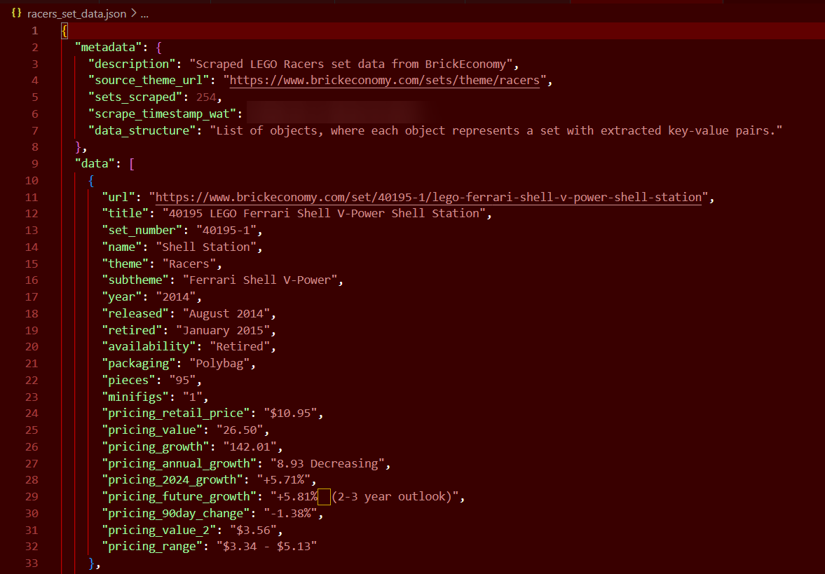
Look at that beautiful, structured data - ready for analysis!
Our image only shows one LEGO set, but don't worry - your JSON will be absolutely packed with brick-based goodness! When you run the full script, you'll capture all 254 sets from the Racers theme in glorious detail. Just imagine scrolling through that JSON file like a LEGO catalog from your childhood, except this one is perfectly structured for data analysis!
And here's a fun bonus - want to scrape a different LEGO theme instead? Simply change the
start_urlvariable to point to any other theme (like "https://www.brickeconomy.com/sets/theme/star-wars" for the Star Wars collection), and you'll be mining a completely different LEGO universe. Just be prepared for a longer coffee break if you tackle the Star Wars theme - with close to 1,000 sets, you might want to pack a lunch!
Analyzing Scraped Data in R: LEGO Price Trends and Value Factors
Now comes the fun part - discovering what our freshly scraped data can tell us! After spending all that time collecting the information, I'm always excited to see what insights are hiding in the numbers. This is where R really shines with its powerful data analysis and visualization capabilities.
Let's load our scraped data and turn it into actionable insights about LEGO Racers sets:
# Load the scraped data
lego_data <- readRDS("racers_set_data.rds")
Before diving into analysis, we need to do some data cleaning. LEGO set data often contains mixed formats:
# Load necessary libraries for analysis
library(dplyr)
library(ggplot2)
library(stringr)
library(tidyr)
library(scales) # For nice formatting in plots
# Clean the pricing and numeric columns
lego_clean <- lego_data %>%
# Convert text columns with numbers to actual numeric values
mutate(
pieces = as.numeric(pieces),
pricing_value = as.numeric(str_remove_all(pricing_value, "[$,]")),
pricing_growth = as.numeric(str_remove_all(pricing_growth, "[+%]")),
pricing_annual_growth = as.numeric(str_remove_all(pricing_annual_growth, "[+%]")),
year = as.numeric(str_extract(year, "\\d{4}"))
) %>%
# Some rows might have NA values after conversion - remove them for analysis
filter(!is.na(pricing_value) & !is.na(pricing_growth))
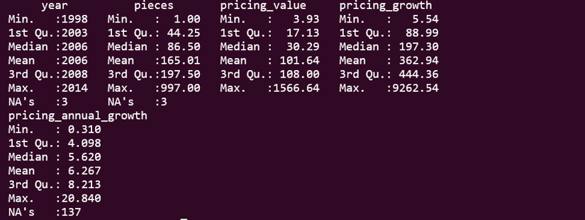
# Check our cleaned data
summary(lego_clean %>% select(year, pieces, pricing_value, pricing_growth, pricing_annual_growth))
Prefer working with spreadsheets? You're not alone! Many data analysts want their scraped data in familiar tools. Check out our guides on scraping data directly to Excel or automating data collection with Google Sheets. These no-code/low-code approaches are perfect when you need to share findings with teammates who aren't R users!
Analysis #1: Which Car Brands See the Largest Average Price Gains?
One of the most interesting questions we can ask about this data is which car brands within the scraped LEGO Racers theme have seen the largest average percentage price gains. Let's find out!
# First, extract car brands from the set titles
# This requires some domain knowledge about car brands
lego_brands <- lego_clean %>%
  mutate(
    brand = case_when(
      str_detect(tolower(title), "ferrari") ~ "Ferrari",
      str_detect(tolower(title), "porsche") ~ "Porsche",
      str_detect(tolower(title), "lamborghini") ~ "Lamborghini",
      str_detect(tolower(title), "mercedes") ~ "Mercedes",
      str_detect(tolower(title), "bmw") ~ "BMW",
      str_detect(tolower(title), "ford") ~ "Ford",
      TRUE ~ "Other"
    )
  )

# Calculate average price gain by brand
brand_growth <- lego_brands %>%
  group_by(brand) %>%
  summarise(
    avg_growth = mean(pricing_growth, na.rm = TRUE),
    avg_annual_growth = mean(pricing_annual_growth, na.rm = TRUE),
    avg_value = mean(pricing_value, na.rm = TRUE),
    count = n()
  ) %>%
  # Only include brands with at least 2 sets for more reliable results
  filter(count >= 2) %>%
  arrange(desc(avg_growth))

# Create a nice table
knitr::kable(brand_growth, digits = 1)
This gives us a clear picture of which brands have appreciated the most.
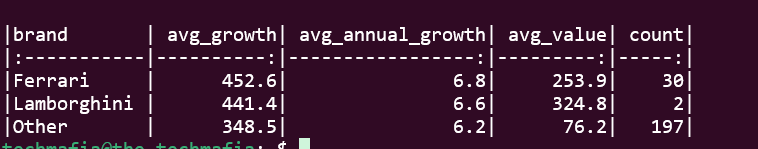
The results are fascinating! As you can see, Ferrari sets emerge as the clear winner in terms of value appreciation, followed by Lamborghini. This makes sense when you think about it - these premium car brands have passionate fan bases both in the real car world and among LEGO collectors.
Analysis #2: How Does Piece Count Influence Value?
Another question we can ask is if piece count correlates with value appreciation. Let's explore this relationship:
# Helper function to remove outliers for better visualization
remove_outliers <- function(df, cols) {
  for (col in cols) {
    q1 <- quantile(df[[col]], 0.025, na.rm = TRUE)
    q3 <- quantile(df[[col]], 0.975, na.rm = TRUE)
    df <- df %>% filter(between(!!sym(col), q1, q3))
  }
  return(df)
}
Now, we clean data for plotting and remove extreme outliers:
# Clean data for plotting - remove extreme outliers
plot_data <- lego_clean %>%
  filter(!is.na(pieces), !is.na(pricing_growth)) %>%
  remove_outliers(c("pricing_growth", "pieces"))

# Create scatter plot - piece count vs growth
piece_plot <- ggplot(plot_data, aes(x = pieces, y = pricing_growth)) +
  geom_point(aes(size = pricing_value, color = year), alpha = 0.7) +
  geom_smooth(method = "lm", se = TRUE, color = "red", linetype = "dashed") +
  scale_y_continuous(labels = function(x) paste0(x, "%")) +
  scale_color_viridis_c() +
  labs(
    title = "Does Piece Count Affect LEGO Racers Value Growth?",
    subtitle = "Exploring the relationship between set size and price appreciation",
    x = "Number of Pieces",
    y = "Price Growth (%)",
    size = "Current Value ($)",
    color = "Release Year"
  ) +
  theme_minimal()

# Display the plot
print(piece_plot)

# Save the plot
ggsave("lego_piece_count_analysis.png", piece_plot, width = 10, height = 6, dpi = 300)
Next, we can calculate correlation between pieces and growth:
# Calculate correlation between pieces and growth
correlation <- cor(plot_data$pieces, plot_data$pricing_growth, use = "complete.obs")
cat("Correlation between piece count and price growth:", round(correlation, 3))

# Run a simple linear model
model <- lm(pricing_growth ~ pieces, data = plot_data)
summary(model)

# Group sets by piece count categories
size_analysis <- lego_clean %>%
  mutate(
    size_category = case_when(
      pieces < 200 ~ "Small (< 200 pieces)",
      pieces < 500 ~ "Medium (200-499 pieces)",
      pieces < 1000 ~ "Large (500-999 pieces)",
      TRUE ~ "Very Large (1000+ pieces)"
    )
  ) %>%
  group_by(size_category) %>%
  summarise(
    avg_growth = mean(pricing_growth, na.rm = TRUE),
    median_growth = median(pricing_growth, na.rm = TRUE),
    avg_value = mean(pricing_value, na.rm = TRUE),
    count = n()
  ) %>%
  # Ensure proper ordering for visualization
  mutate(size_category = factor(size_category,
                               levels = c("Small (< 200 pieces)",
                                         "Medium (200-499 pieces)",
                                         "Large (500-999 pieces)",
                                         "Very Large (1000+ pieces)"))) %>%
  arrange(size_category)
Finally, we can create a bar chart for size categories:
# Create a bar chart for size categories
size_plot <- ggplot(size_analysis, aes(x = size_category, y = avg_growth, fill = size_category)) +
  geom_bar(stat = "identity") +
  geom_text(aes(label = paste0(round(avg_growth, 1), "%")),
            position = position_stack(vjust = 0.5), color = "white") +
  scale_y_continuous(labels = function(x) paste0(x, "%")) +
  labs(
    title = "Average Growth by LEGO Set Size",
    subtitle = "How piece count correlates with value appreciation",
    x = "Size Category",
    y = "Average Growth (%)"
  ) +
  theme_minimal() +
  theme(legend.position = "none",
        axis.text.x = element_text(angle = 45, hjust = 1))

# Display the second plot
print(size_plot)

# Save the second plot
ggsave("lego_size_category_analysis.png", size_plot, width = 10, height = 6, dpi = 300)

# Create a nice table
knitr::kable(size_analysis, digits = 1)
As you can see in your directory, the script will create lego_piece_count_analysis.png - The scatter plot showing the relationship between piece count and growth:
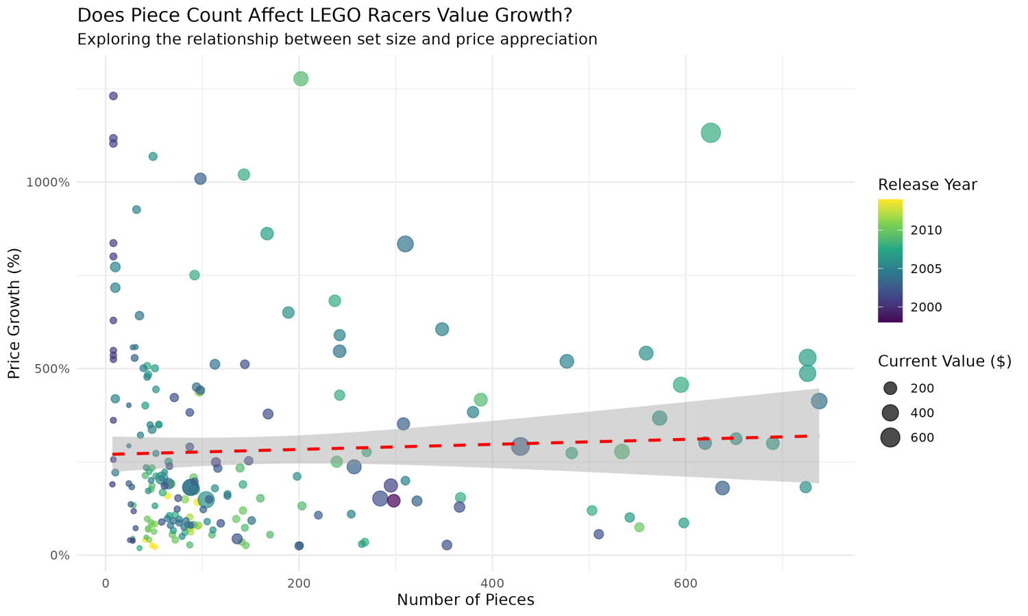
Similarly, we've lego_size_category_analysis.png - The bar chart comparing growth across different size categories:

My results might surprise you:
- Correlation Analysis: With a correlation of 0.045 and a high p-value (0.526), there is essentially no significant relationship between piece count and price growth. The piece count alone doesn't seem to predict value appreciation.
- Size Category Findings:
- Very large sets (1000+ pieces) show extraordinary growth (811.9%), but with only 3 sets, this is not statistically reliable
- Small sets (< 200 pieces) actually show the next highest growth at 371.8%
- Medium and large sets show similar growth rates (around 308-316%)
- Interesting Insight: The highest growth in both the smallest and largest categories suggests a "barbell strategy" might work for LEGO investors - focusing on either very small or very large sets.
These insights demonstrate the power of web scraping combined with R's data analysis capabilities. We've gone from raw HTML to actionable investment advice for LEGO collectors!
Scaling Up: When Your R Script Needs Superpowers (Enter ScrapingBee!)
So, we did it! After navigating tricky JavaScript pagination and finally wrestling the details out of advanced individual pages, we have our LEGO Racers dataset. High fives all around! It was quite the journey, wasn't it? From lengthy functions to chromote's mysterious loops of despair and finally landing the data (hopefully!).
But let's be real. While our R chromote solution is elegant for personal projects, it comes with some real-world limitations:
- IP Blocking Risk: After running our scraper a few times, I noticed BrickEconomy started getting suspicious. One more scraping session and we might get our IP address blocked.
- Maintenance Nightmares: Websites change their structure constantly. Remember how we carefully crafted those CSS selectors? They could break tomorrow.
- Scaling Challenges: Want to scrape 10,000 pages instead of 250? Good luck managing all those browser instances and network requests without crashing your system.
Now, this is the question: "Is maintaining your own scraping infrastructure really the best use of your time?"
What if you could skip the headaches? Imagine just asking for the data you need in plain English, without wrestling with selectors or headless browser quirks.
Forget CSS Selectors - Use AI! This is the game-changer. Instead of meticulously finding and maintaining CSS selectors (which break the moment a website redesigns), we now offer an AI Web Scraping API:
You simply describe the data you want in plain English (e.g., "Extract the set name, current value, retail price, and piece count for this LEGO set page"), and our AI Web Scraping API figures out where that data is and returns it structured, usually as JSON. It adapts to layout changes automatically!
Ready to supercharge your web scraping? Get started with 1,000 free API calls - no credit card required.
Further Reading: Check Out Web Scraping in Other Languages
Think R is the only language in our web scraping arsenal? Think again! Whether you're a polyglot programmer or just curious about alternatives, we've got comprehensive guides on how to tackle web scraping using other popular languages:
| Article | Description |
|---|---|
| Web Scraping with Python | The crowd favorite! Learn scraping with Python's powerful libraries. Like R but with more snakes and fewer arrows. |
| Web Scraping with PHP | Because sometimes you need to extract data and generate HTML all in one go. The Swiss Army knife of server-side scraping. |
| Web Scraping with Perl | The original web scraping language! For those who enjoy regular expressions a bit too much. |
| Web Scraping with Rust | When you absolutely, positively need to extract every bit of data as fast as humanly possible. Speed demons only! |
| Web Scraping with Go | Concurrency meets simplicity. Perfect for scraping 10,000 pages before your coffee gets cold. |
| Web Scraping with Java | Enterprise-grade scraping with type safety. Because sometimes a 20-line script should really be 200 lines with proper design patterns. |
Wheew, what a day! Our time with R web scraping comes to an end. We saw how powerful R can be, using tools like rvest for parsing and advanced browser automation packages for handling heavy JavaScript.
Hopefully, this journey equips you with code snippets and a better understanding of the process: the importance of inspection, the different tools available, the challenges you might face, and when it might be time to call our AI-powered web scraping API with its advanced features.
Happy scraping!